모델의 성능을 높이고, 오버피팅을 방지하는 Regularization과 Nomalizaton을 알아보자
Regularization : 정칙화
- L1, L2 Regularization, Dropout, Batch normalization 등이 있음
- 모델이 train set의 정답을 맞히지 못하도록 오버피팅을 방해(train loss가 증가) 하는 역할
- train loss는 약간 증가하지만 결과적으로, validation loss나 최종적인 test loss를 감소시키려는 목적
Normalization : 정규화
- 데이터의 형태를 좀 더 의미 있게, 혹은 트레이닝에 적합하게 전처리하는 과정
- 데이터를 z-score로 바꾸거나 minmax scaler를 사용하여 0과 1사이의 값으로 분포를 조정하는 것들이 해당
- 모든 피처의 범위 분포를 동일하게 하여 모델이 풀어야 하는 문제를 좀 더 간단하게 바꾸어 주는 전처리 과정
Iris dataset의 회귀 문제 풀며 regularizatiion, nomalization 비교해 보기
from sklearn.datasets import load_iris
import pandas as pd
import matplotlib.pyplot as plt

iris = load_iris()
iris_df = pd.DataFrame(data=iris.data, columns=iris.feature_names)
target_df = pd.DataFrame(data=iris.target, columns=['species'])

# 0, 1, 2로 되어있는 target 데이터를
# 알아보기 쉽게 'setosa', 'versicolor', 'virginica'로 바꿉니다
def converter(species):
    if species == 0:
        return 'setosa'
    elif species == 1:
        return 'versicolor'
    else:
        return 'virginica'

target_df['species'] = target_df['species'].apply(converter)

iris_df = pd.concat([iris_df, target_df], axis=1)
iris_df.head()
결과

Iris data 중 virginica라는 종의 petal length(꽃잎 길이)를 X, sepal length(꽃받침의 길이)를 Y로 두고 print
X = [iris_df['petal length (cm)'][a] for a in iris_df.index if iris_df['species'][a]=='virginica']
Y = [iris_df['sepal length (cm)'][a] for a in iris_df.index if iris_df['species'][a]=='virginica']

print(X)
print(Y)
결과
[6.0, 5.1, 5.9, 5.6, 5.8, 6.6, 4.5, 6.3, 5.8, 6.1, 5.1, 5.3, 5.5, 5.0, 5.1, 5.3, 5.5, 6.7, 6.9, 5.0, 5.7, 4.9, 6.7, 4.9, 5.7, 6.0, 4.8, 4.9, 5.6, 5.8, 6.1, 6.4, 5.6, 5.1, 5.6, 6.1, 5.6, 5.5, 4.8, 5.4, 5.6, 5.1, 5.1, 5.9, 5.7, 5.2, 5.0, 5.2, 5.4, 5.1]
[6.3, 5.8, 7.1, 6.3, 6.5, 7.6, 4.9, 7.3, 6.7, 7.2, 6.5, 6.4, 6.8, 5.7, 5.8, 6.4, 6.5, 7.7, 7.7, 6.0, 6.9, 5.6, 7.7, 6.3, 6.7, 7.2, 6.2, 6.1, 6.4, 7.2, 7.4, 7.9, 6.4, 6.3, 6.1, 7.7, 6.3, 6.4, 6.0, 6.9, 6.7, 6.9, 5.8, 6.8, 6.7, 6.7, 6.3, 6.5, 6.2, 5.9]
산점도 그려보기
plt.figure(figsize=(5,5))
plt.scatter(X,Y)
plt.title('petal-sepal scatter before normalization')
plt.xlabel('petal length (cm)')
plt.ylabel('sepal length (cm)')
plt.grid()
plt.show()
결과

아직 Nomalization은 하지 않았기 때문에, 최솟값과 최댓값의 범위로 그려짐
0~1로 nomalization해줌 - minmax_scale
from sklearn.preprocessing import minmax_scale

X_scale = minmax_scale(X)
Y_scale = minmax_scale(Y)

plt.figure(figsize=(5,5))
plt.scatter(X_scale,Y_scale)
plt.title('petal-sepal scatter after normalization')
plt.xlabel('petal length (cm)')
plt.ylabel('sepal length (cm)')
plt.grid()
plt.show()
결과

분포는 변하지 않고, 축 범위가 0~1로 rescale된 것을 확인할 수 있다. - x,y의 관계 다루기 용이해짐
회귀문제 풀어보기 - Linear Regression 모델 이용
from sklearn.linear_model import LinearRegression
import numpy as np

X = np.array(X)
Y = np.array(Y)

# Iris Dataset을 Linear Regression으로 학습합니다.
linear= LinearRegression()
linear.fit(X.reshape(-1,1), Y)

# Linear Regression의 기울기와 절편을 확인합니다.
a, b=linear.coef_, linear.intercept_
print("기울기 : %0.2f, 절편 : %0.2f" %(a,b))
결과
기울기 : 1.00, 절편 : 1.06일차함수 회귀선과 함께 산점도 그려보기
plt.figure(figsize=(5,5))
plt.scatter(X,Y)
plt.plot(X,linear.predict(X.reshape(-1,1)),'-b')
plt.title('petal-sepal scatter with linear regression')
plt.xlabel('petal length (cm)')
plt.ylabel('sepal length (cm)')
plt.grid()
plt.show()
결과

L1 regularization인 Lasso로 문제 풀기
#L1 regularization은 Lasso로 import 합니다.
from sklearn.linear_model import Lasso

L1 = Lasso()
L1.fit(X.reshape(-1,1), Y)
a, b=L1.coef_, L1.intercept_
print("기울기 : %0.2f, 절편 : %0.2f" %(a,b))

plt.figure(figsize=(5,5))
plt.scatter(X,Y)
plt.plot(X,L1.predict(X.reshape(-1,1)),'-b')
plt.title('petal-sepal scatter with L1 regularization(Lasso)')
plt.xlabel('petal length (cm)')
plt.ylabel('sepal length (cm)')
plt.grid()
plt.show()
결과
기울기 : 0.00, 절편 : 6.59
기울기가 0으로 나옴 - Lasso 방법은 제대로 문제를 풀지 못함!
L2 regularization인 Ridge로 문제를 풀기
#L2 regularization은 Ridge로 import 합니다.
from sklearn.linear_model import Ridge

L2 = Ridge()
L2.fit(X.reshape(-1,1), Y)
a, b = L2.coef_, L2.intercept_
print("기울기 : %0.2f, 절편 : %0.2f" %(a,b))

plt.figure(figsize=(5,5))
plt.scatter(X,Y)
plt.plot(X,L2.predict(X.reshape(-1,1)),'-b')
plt.title('petal-sepal scatter with L2 regularization(Ridge)')
plt.xlabel('petal length (cm)')
plt.ylabel('sepal length (cm)')
plt.grid()
plt.show()
결과
기울기 : 0.93, 절편 : 1.41
L2 Regularization을 쓰는 Ridge방법으로는 앞서 Linear Regression과 큰 차이가 없는 결과가 나옴
L1 Regularization
정의


p = 1 인 경우 해당 L1 norm의 식이 lasso 식의 마지막 항과 일치 -> L1 regularization이라고 부르는 이유!
이전 스텝에서 왜 L1 Regularization 만 회귀선이 제대로 그려지지 않은 이유?

를 petal length, Y를 sepal length로 하여 N=50, p=1인 선형 회귀 가짐, 는 절편, 은 기울기
기울기나 절편에 대해 최댓값, 최솟값을 구하기 위해 미분을 해보자.
기울기 β1에 대해 해당 식을 미분하면

과 같은 결과가 나온다
또한, 절편 β0에 대해 해당 식을 미분하면

과 같은 결과가 나온다.
p=1인 경우 β0으로 미분하는 과정에서 가 사라지므로(β0가 항에 없으므로 상수항 취급되어 미분시 0으로 사라짐) Regularization의 효과를 볼 수 없다.
와인 데이터셋으로 L1 regularization 확인하기
컬럼수가 13개인 와인데이터로 확인해보기
데이터 가져오기
from sklearn.datasets import load_wine

wine = load_wine()
wine_df = pd.DataFrame(data=wine.data, columns=wine.feature_names)
target_df = pd.DataFrame(data=wine.target, columns=['Y'])

wine_df.head(5)
target_df.head(5)
Linear regression 으로 문제를 풀고, 그 계수(coefficient)와 절대 오차(mean absolute error), 제곱 오차(mean squared error), 평균 제곱값 오차(root mean squared error)를 출력
from sklearn.model_selection import train_test_split
from sklearn.linear_model import LinearRegression
from sklearn.metrics import mean_absolute_error, mean_squared_error

# 데이터를 준비하고
X_train, X_test, y_train, y_test = train_test_split(wine_df, target_df, test_size=0.3, random_state=101)

# 모델을 훈련시킵니다.
model = LinearRegression()
model.fit(X_train, y_train)

# 테스트를 해볼까요?
model.predict(X_test)
pred = model.predict(X_test)

# 테스트 결과는 이렇습니다!
print("result of linear regression")
print('Mean Absolute Error:', mean_absolute_error(y_test, pred))
print('Mean Squared Error:', mean_squared_error(y_test, pred))
print('Mean Root Squared Error:', np.sqrt(mean_squared_error(y_test, pred)))

print("\n\n coefficient linear regression")
print(model.coef_)
결과
result of linear regression
Mean Absolute Error: 0.25128973939722626
Mean Squared Error: 0.1062458740952556
Mean Root Squared Error: 0.32595379134971814


 coefficient linear regression
[[-8.09017190e-02  4.34817880e-02 -1.18857931e-01  3.65705449e-02
  -4.68014203e-04  1.41423581e-01 -4.54107854e-01 -5.13172664e-01
   9.69318443e-02  5.34311136e-02 -1.27626604e-01 -2.91381844e-01
  -5.72238959e-04]]
L1 regularization으로 문제를 풀기
from sklearn.linear_model import Lasso
from sklearn.metrics import mean_absolute_error, mean_squared_error

# 모델을 준비하고 훈련시킵니다.
L1 = Lasso(alpha=0.05)
L1.fit(X_train, y_train)

# 테스트를 해봅시다.
pred = L1.predict(X_test)

# 모델 성능은 얼마나 좋을까요?
print("result of Lasso")
print('Mean Absolute Error:', mean_absolute_error(y_test, pred))
print('Mean Squared Error:', mean_squared_error(y_test, pred))
print('Mean Root Squared Error:', np.sqrt(mean_squared_error(y_test, pred)))

print("\n\n coefficient of Lasso")
print(L1.coef_)
결과
result of Lasso
Mean Absolute Error: 0.24233731936122138
Mean Squared Error: 0.0955956894578189
Mean Root Squared Error: 0.3091855259513597


 coefficient of Lasso
[-0.          0.01373795 -0.          0.03065716  0.00154719 -0.
 -0.34143614 -0.          0.          0.06755943 -0.         -0.14558153
 -0.00089635]
결과분석
- Linear Regression에서는 모든 컬럼의 가중치를 탐색하여 구하는 반면, L1 Regularization에서는 총 13개 중 7개를 제외한 나머지의 값들이 모두 0
- Error 부분에서는 큰 차이가 없었지만, L1에선 어떤 컬럼이 결과에 영향을 더 크게 미치는지 확실히 확인할 수 있음
- 다른 문제에서도 error의 차이가 크게 나지 않는다면, 차원 축소와 비슷한 개념으로 변수의 값을 7개만 남겨도 충분히 결과를 예측할 수 있다는 뜻
- Linear Regression과 L1, L2 Regularization의 차이 중 하나는 λ라는 하이퍼파라미터가 하나 더 들어간다는 것이고, 그 값에 따라 error에 영향을 미친다는 점
L2 Regularization

L1 / L2 Regularization의 차이점

- L1 Regularizaion(Lasso)는 를 이용하여 마름모 형태의 제약조건이 생김
- 위의 등고선처럼 보이는 내용은 우리가 풀어야 하는 문제. 이 문제가 제약조건과 만나는 지점이 해가 된다
- L2 regularization은 이므로 원의 형태 - 제곱이 들어가 있기 때문에 절댓값으로 L1 Norm을 쓰는 Lasso보다는 수렴이 빠르다는 장점 有
L2 regularization으로 문제를 풀기
from sklearn.linear_model import Ridge

L2 = Ridge(alpha=0.05,max_iter=5)
L2.fit(X_train, y_train)
pred = L2.predict(X_test)

print("result of Ridge")
print('Mean Absolute Error:', mean_absolute_error(y_test, pred))
print('Mean Squared Error:', mean_squared_error(y_test, pred))
print('Mean Root Squared Error:', np.sqrt(mean_squared_error(y_test, pred)))

print("\n\n coefficient of Ridge")
print(L2.coef_)
결과
result of Ridge
Mean Absolute Error: 0.251146695993643
Mean Squared Error: 0.10568076460795564
Mean Root Squared Error: 0.3250857803841251


 coefficient of Ridge
[[-8.12456257e-02  4.35541496e-02 -1.21661565e-01  3.65979773e-02
  -3.94014013e-04  1.39168707e-01 -4.50691113e-01 -4.87216747e-01
   9.54111059e-02  5.37077039e-02 -1.28602933e-01 -2.89832790e-01
  -5.73136185e-04]]
선형 회귀 linear regression과 같은 값이 나오는 L2
정리
- L1 Regularization은 가중치가 적은 벡터에 해당하는 계수를 0으로 보내면서 차원 축소와 비슷한 역할을 하는 것이 특징
- L2 Regularization은 0이 아닌 0에 가깝게 보내지만 제곱 텀이 있기 때문에 L1 Regularization보다는 수렴 속도가 빠르다는 장점
- A=[1,1,1,1,1], B=[5,0,0,0,0] 의 경우 L1-norm은 같지만, L2-norm은 같지 않다. 즉, 제곱 텀에서 결과에 큰 영향을 미치는 값은 더 크게, 결과에 영향이 적은 값들은 더 작게 보내면서 수렴 속도가 빨라지는 것
데이터에 따라 적절한 Regularization 방법을 활용하는 것이 좋다.
Lp norm
Norm이라는 개념은 벡터뿐만 아니라 함수, 행렬에 대해서 크기를 구하는 것
vector norm


matrix norm

Dropout
- 확률적으로 랜덤하게 몇 가지의 뉴럴만 선택하여 정보를 전달하는 과정
- 오버피팅을 막는 Regularization layer 중 하나 - train을 방해해 train accuracy는 떨어지나 val accuracy는 증가
- 확률을 너무 높이면, 제대로 전달되지 않으므로 학습이 잘되지 않고, 확률을 너무 낮추는 경우는 fully connected layer와 동일해져 효과 X
https://keras.io/api/layers/regularization_layers/dropout/
Keras documentation: Dropout layer
Dropout layer Dropout class tf.keras.layers.Dropout(rate, noise_shape=None, seed=None, **kwargs) Applies Dropout to the input. The Dropout layer randomly sets input units to 0 with a frequency of rate at each step during training time, which helps prevent
keras.io
Batch Normalization
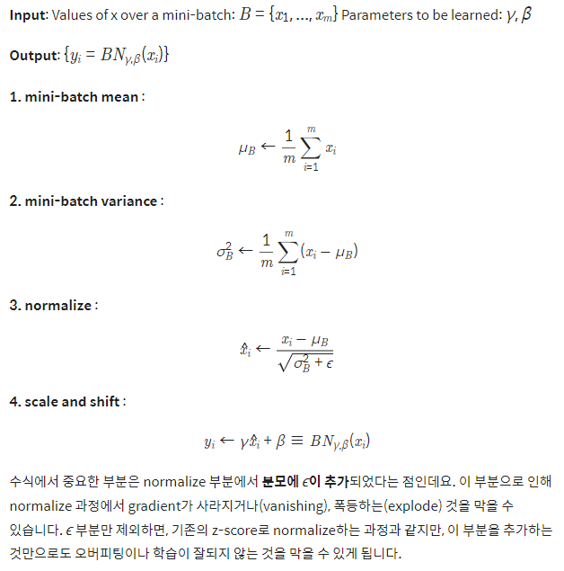
- 학습에 Batch Normalization을 추가하니 좀 더 빠르게 정확도 상승이 있음이 확인됨.
- 또한 loss 함수의 감소도 더 빨라짐을 확인.
- Batch Normalization으로 인해 이미지가 정규화되면서 좀 더 고른 분포를 가지기도 하며, 부분으로 인해 안정적인 학습이 가능
'Computer Technology 기록부 > 인공지능 학습 기록부' 카테고리의 다른 글
| Image Data Generation using DCGAN(ENG) (0) | 2023.02.06 |
|---|---|
| Iris Data Classification Report(ENG) (0) | 2023.02.06 |
| 딥러닝 레이어 이해하기 Embedding Layer, Recurrent layer (0) | 2022.02.09 |
| 딥러닝 레이어 이해하기 linear, Convolution (0) | 2022.02.08 |
| Deep network 종류 (0) | 2022.02.08 |


댓글