Iris Classification Project
Purpose
1. To build and train a machine learning model that classifies iris data.
2. To creates an optimal classification model through numerical data analysis and preprocessing, various model learning, and result analysis. It is expected that the results of learning and analysis will not be clear due to the small amount of data.
What is Iris dataset?
This data sets consists of 3 different types of irises’ (Setosa, Versicolour, and Virginica) petal and sepal length, stored in a 150x4 numpy.ndarray. The rows being the samples and the columns being: Sepal Length, Sepal Width, Petal Length and Petal Width.

1. Data Analysis
The Sklearn library offer many useful methods. For Iris dataset, we can also use various methods. You can easily download the iris dataset with this code once you import the Sklearn package.
from sklearn.datasets import load_iris

iris = load_iris()
Size/Feature of Data
| Classes | 3 |
| Sample per class | 50 |
| Sample total | 150 |
| Dimensionality | 4 |
| Features | Real, Positive |
We can see the size with these methods. The size of data is 150 X 4 and the target is 150 X 1. The 3 classes called Setosa, Versicolor, Viginica. The 4 features are Sepal width, Sepal length, Petal width, and Petal length.
Distribution/Relationship between each feature
To find out the data distribution between each feature, I visualized it using the hist plot of the seaborn library. As you can see, a normal distribution is confirmed in the Sepal length and Sepal width. 50 labels were the same for each class, confirming that there is no data imbalance problem. In the Petal features, it was confirmed that the data were not evenly distributed and gathered in a specific interval. This gap may help with classification.
As we can see in the plot, each class are the dataset with distinct characteristics. In this case, even a simple machine learning algorithm will be able to produce a sufficiently high performance.
2. Data Preprocessing for Machine Learning
Data Cleaning: Remove the Outlier
To better training, we need to do data cleaning. Fortunately, there are no missing values in the data, so I decided to deal with outlier data only. The criteria for defining outlier data were set as IQR method.
IQR method
The quartiles of a ranked set of data values are three points which divide the data into exactly four equal parts, each part comprising of quarter data.
- Q1 is defined as the middle number between the smallest number and the median of the data set.
- Q2 is the median of the data.
- Q3 is the middle value between the median and the highest value of the data set.
- IQR is Q3 - Q1
|
Original data(left), Data after remove the outlier(right)
|
Values greater than (Q3+1.5*IQR) and values less than (Q1-1.5*IQR)) are defined as outliers. To visualize, let’s create the box plot for each feature.
Only in Sepal width, there are 4 outliers. These outliers will cause harmful effect while training the model. I deleted it by using the where method in numpy and drop in pandas.
After Processing: Final Dataset Visualization
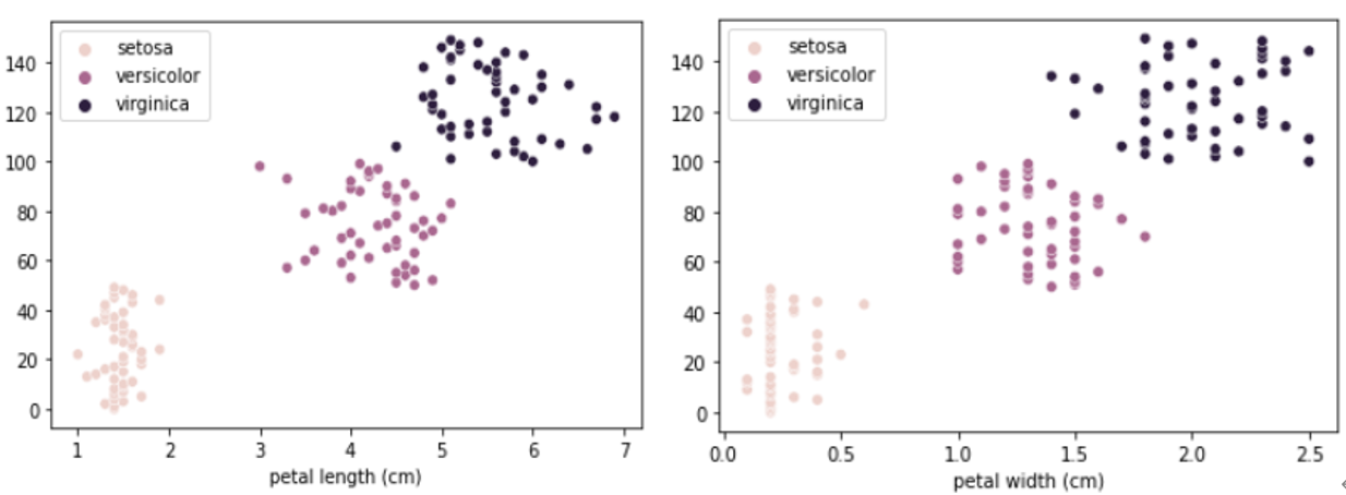
In these scatter plots, the x-axis is drawn with each feature and the y-axis with the index of the data. Through this visualization plot, we can see the distribution of data was relatively clustered according to iris species.
3. Data Split – train and test
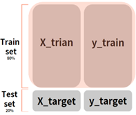
We need to split the data set to create a training set and a test set. You should only train on the training set, not the test set. Otherwise, the model will overfit the entire data and its accuracy will be unreliable. In machine learning, we usually test the accuracy of a model by creating a validation set as well as a training set and a test set. This allows us to measure accuracy without using a test set while preventing the model from overfitting the training data. However, I will not be using a validation set for this project. Instead, a cross-validation technique will be used.
Cross Validation: No validation set
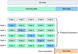
Cross-validation is a technique that randomly extracts data from a training set and uses it as a validation set without using a validation set. For each training session, a different part of the data set is extracted and designated as the validation set. After training with only the remaining data, the model calculates a score through a specified validation set. After that, data is extracted from other parts, calculated as a validation set, and learning is performed with data excluding that part. and calculates the score. After repeating this process several times (usually 5 times), the final score is calculated as the average value of the calculated scores.
Split with train_test_split method in sklearn
With sklearn train_test_split method, we can easily split the dataset to trainset and test set. The test set was calculated as 20 percent of the entire data set. Since the data is small, separating too much data into the test set risks underfitting. Below is the method for split the data.
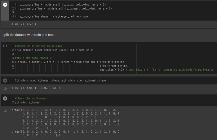
Imbalance Problem
But here for a moment let's look at the distribution of classes within the train set and test set. Are all three classes equally present? Let's check it through the function.
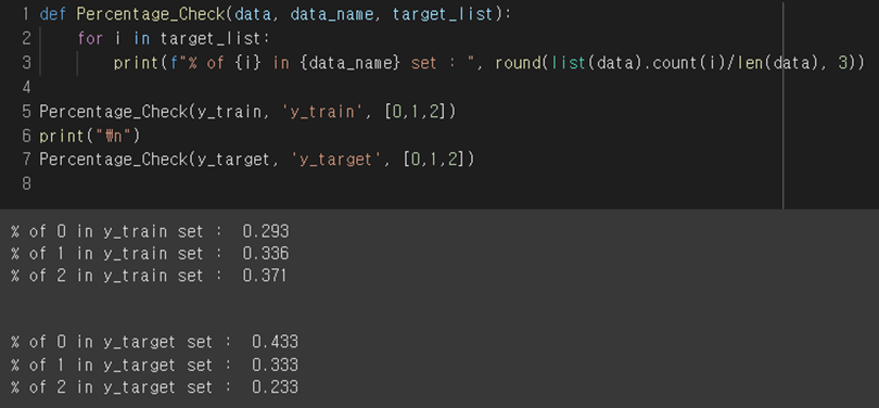
As a result of checking, the class distribution came out unbalanced in both the training set and the test set. This means that it is trained with an imbalanced data set, which can have severe effects on training.
Stratified Sampling
Purely random sampling methods are generally fine if the dataset is large enough, but if it's not, then we run the risk of introducing a significant sampling bias. I will use stratified sampling: When this method divides the training set and the test set, the ratio of each class is divided equally.
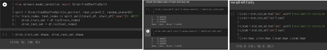
The codes to split the data with Stratified method, class ratio after split the data, split each dataset with X and y
4. Training model
As a result of data analysis, it is predicted that more basic machine learning classification models will produce better results than deep learning models, considering that the data size is small, the number of data per class is the same, and the difference between classes for each feature is prominent. Therefore, we will perform classification tasks using machine learning models such as SVM, Decision Tree, RF, and KNN. In addition, ensemble learning, and deep learning will also be used to compare the results.
4-1. SVM
What is SVM?
The SVM is a versatile machine learning model that can be used for linear or nonlinear classification, regression, and outlier detection. SVMs are particularly well suited to complex classification problems, but do not work well with large data sets.
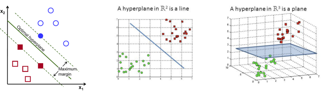
The objective of the support vector machine algorithm is to find a hyperplane in an N-dimensional space (N — the number of features) that distinctly classifies the data points.
Since the Iris dataset can be considered as a small dataset, I think using SVM is suitable for this task.
Parameters in SVM
There are numerous parameters in SVM. SVMs have numerous parameters. The parameters below have the greatest impact on SVM performance.
- Kernel: Specifies the kernel type to be used in the algorithm.
- Gamma: Adjust the range of data that affects the curvature of the decision boundary. The smaller the gamma, the smaller the range.
- C: Regularization parameter. Controls tradeoff between smooth decision boundary and classifying training points correctly. If C is small, decision boundary become more like straight line. If C is big, decision boundary will get more fluctuation.
Visualization SVM decision boundary by each Kernel
SVM is basically a linear classification technique using a hyperplane, but in order to solve this problem when linear classification is not possible, it maps low-dimensional data to high-dimensional data through a kernel function as shown in the figure below to enable linear classification. I was curious to see how much difference there was in classification performance depending on these kernels, so I decided to compare them.
Result Analysis
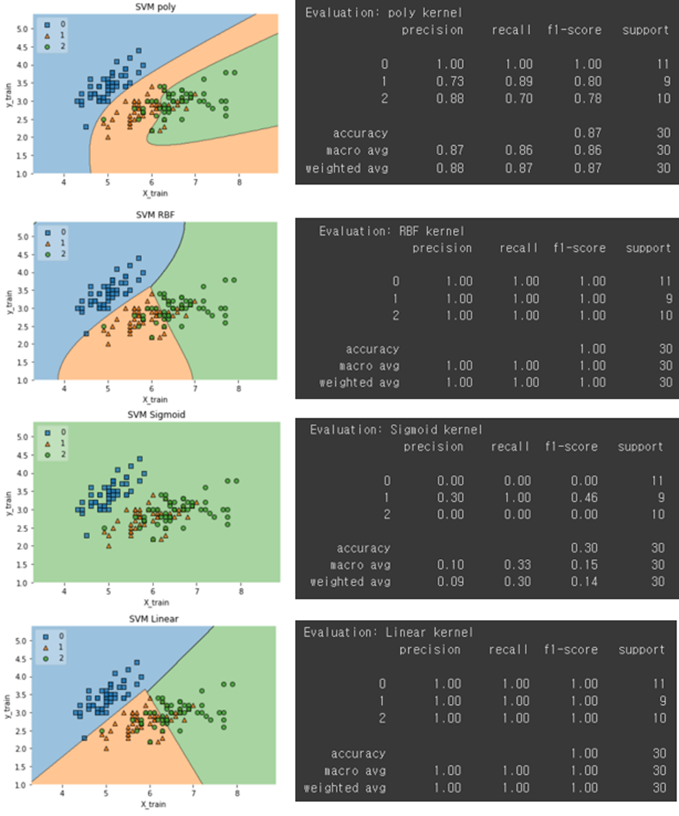
All hyper parameters are fixed to experiment except Kernel type. Most of the models recorded 100% accuracy. I believe that this is not overfitting, but a problem caused by the data set being too small. This problem occurs because only 20 percent of the entire dataset, that is, 30 data, is separated into the test set. Using a larger data set or increasing the percentage of the test set will reduce it slightly from 100 percent. However, since the data set is also small, having a larger proportion of the test set makes the training data too small. So, I don't think that's a good way.
All kernels work well, but not in sigmoid kernel. This is due to the reason that sigmoid function returns two values, 0 and 1, therefore it is more suitable for binary classification problems. However, in our case we had three output classes. Therefore, Sigmoid kernel doesn’t work in multi class classification.
Grid Search for SVM
From now on, I will tune the SVM hyper parameter with Grid Search method. I chose the Gamma, C, and Kernel. The table below is the result of grid search with pandas data frame. I sorted the results with the Cross-validation mean test score.
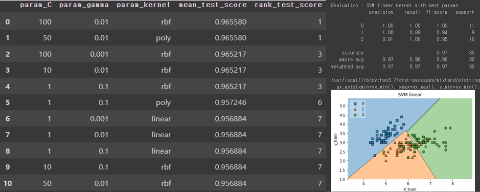
The best parameters were C = 100, gamma = 0.01, kernel = RBF. The accuracy of this model is 97%. The default model with gamma = auto is better than best parameters combination model.
4-2. Decision tree / Random Forest (RF)
What is Decision tree?
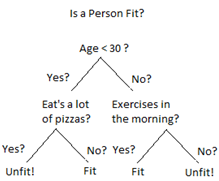
Decision Trees are a type of Supervised Machine Learning (that is you explain what the input is and what the corresponding output is in the training data) where the data is continuously split according to a certain parameter. The tree can be explained by two entities, namely decision nodes and leaves. The leaves are the decisions or the final outcomes. The decision nodes are where the data is split. It usually used for classification and regression. The advantages of decision trees are simple to understand and to interpret and doesn’t need a high computing power. Moreover, it doesn’t need any data scaling and for training. This mean it will work well with our original data, too.
Parameters in Decision tree
- Criterion: The function to measure the quality of a split. “gini” for the Gini impurity and “log_loss” and “entropy” both for the Shannon information gain
- Max_depth: The maximum depth of the tree. If None, then nodes are expanded until all leaves are pure or until all leaves contain less than min_samples_split samples
- Min_sample_leaf: The minimum number of samples required to be at a leaf node.
- Min_samples_split: The minimum number of samples required to split an internal node
- Splitter: The strategy used to choose the split at each node. Supported strategies are “best” to choose the best split and “random” to choose the best random split
Grid Search for decision tree
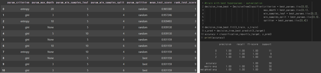
From now on, I will tune the Decision tree hyper parameter with Grid Search method. I chose the Criterion, Min_sample_leaf, Splitter, and Max_depth. The table below is the result of grid search with pandas data frame. I sorted the results with the Cross-validation mean test score. However, we must consider that decision trees are very susceptible to overfitting. Even if the accuracy is high, it may be that the accuracy is overfitting even on the test set. Given new data, we must consider the possibility that the model will make a wrong decision.
Result Analysis
Model with criterion = entropy, max_depth = 20, min_samples_leaf = 5, min_sample_split = 6, splitter = random got highest score in mean test score.
In the top 10, most of the models using spitter = random occupied the place. If the model use random splitter, the model if taking the feature randomly but with the same distribution. In other words, instead of testing every possible threshold for the split on a feature, a single random threshold, drawn uniformly between the feature's minimum and maximum, is tested.
What is Random Forest?

Earlier, we learned that decision trees are vulnerable to overfitting. So how can we prevent it? The answer is to use random forest, one of the ensembles learning methods. A random forest is an ensemble of decision trees generally using a bagging method. Random forest is a model that trains several decision trees and calculates the final result by combining the result values from each classifier. Because the results from multiple models are combined, overfitting can be prevented, and generalization performance can be improved.
Result Analysis
The left picture is result of Random Forest Classifier. Since I didn’t modify the parameters, the model will run with default parameters. The default number of estimator is 100, which means this classifier will train 100 different Decision Tree and aggregating all result together. The accuracy decreased a bit, due to the model generalized more.
4-3. K-NN
What is K-NN?
The k-nearest neighbors algorithm, also known as KNN or k-NN, is a non-parametric, supervised learning classifier, which uses proximity to make classifications or predictions about the grouping of an individual data point.
In Scikit-learn, K-NN classifier does not attempt to construct a general internal model, but simply stores instances of the training data.
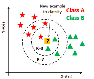
Parameter K in K-NN
K is a parameter that refers to the number of nearest neighbors to include in the majority of the voting process. If K is 3, the model checks the nearest 3 datapoint from input. Within 3 data points, the model yields the most frequently occurring class as the correct answer.
Experiment with various K value ( K = 1, 3, 5); How to set K value?
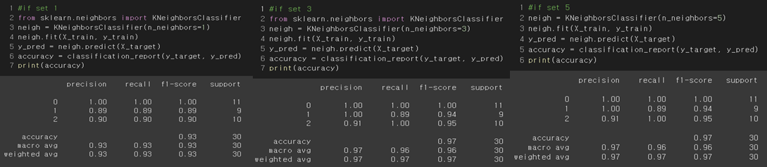
Result Analysis
I experimented with K = 1, 3, and 5. Result was highest when K was 3 or 5, and it was lowest when K was 1. When we set the K, it is not a great idea to set K as smaller than number of class when the data has lots of noise. It has a big risk to get overfitting problem. Moreover, even though the result in this dataset was same either k = 3 or k = 5 as 97% of accuracy, it is safer to use k = 5. The reason why k = 5 is safer than k =3 is because there are 3 classes in this dataset. If the classes of the three nearest data points are all different, the model with K = 3 may make an error in selecting the correct answer. Therefore, it seems safer to set k = 5, which is 1 higher than the number of classes, so that ties never occur. (Also, it is odd number)
4-4. Deep Learning Algorithms
Although this data is too simple and small to use deep learning algorithms, let’s try to train basic MLP and CNN model.
MLP
First, we will use Multi-Layer Perceptron. This is the most basic deep learning model with dense layers for hidden layers.
Modified structure
- Delete the Flatten layer: Since our datapoint is already 1 dimension (4 X 1 for 1 data), we do not need flatten layer for the first layer in MLP. The input will directly get into Dense layer.
- Change the output size to 3 due to the number of classes.
- fix the metrics as accuracy to compare with other model’s results.
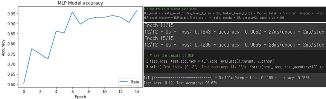
Training score/ Test accuracy
The model trained well with train dataset and return 96.67% of accuracy with the test data. Although there was no validation set, which means it has high possibility to have overfitting, the test accuracy is quite reliable.
CNN
CNN is the convolution neural network, the most common and famous for Computer Vision field. This model shows excellent performance mainly for processing images or videos, but we will also apply it to the corresponding iris data set.
Modified structure
- Using Conv1D layer for hidden layer: To receive the input of a 1D array, we must replace it with a 1D convolution layer.
- Change input shape as (4,1)
- Change output layer’s size as 3: Since we have 3 classes in this data, we must change the output layer size as 3.
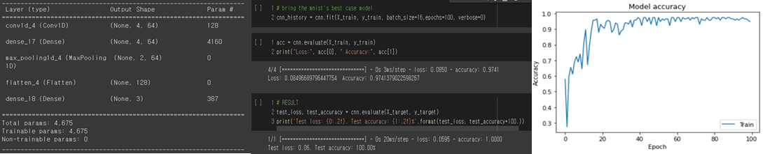
Model structure/Training Score/Test accuracy
4-5. Ensemble Learning
An ensemble learning model combines the predictions from two or more models. The models that contribute to the ensemble, referred to as ensemble members, may be the same type or different types and may or may not be trained on the same training data. The goal of ensemble methods is to combine the predictions of several base estimators built with a given learning algorithm in order to improve generalizability / robustness over a single estimator.
Bagging/Boosting/stacking methods
There are 3 ways to doing ensemble learning.
- Bagging: Using different subsets of the data or features (or both) are used to generate different scores. The ensembled models will same type of classifier, and same parameters. Score function supposed to be same too.
- Boosting: The idea of the boosting method is to learn a set of predictors by complementing the previous model. Using different type of classifiers. Usually, we say different classifiers when parameters in classifiers are different. The score function supposed to be same.
- Stacking: Using different subsets of data or features, and using different type of classifiers, such as decision tree, SVM, KNN, etc. Even the scoring function is different. Metaclassifier will be used to combine the all-model’s score.
Bagging Classifier
Bagging method is used to build high-level generalized models. Let’s use it to our data to generalize the model. I will use bagging with KNN and SVC classifier.
Parameters in Bagging Classifier
- n_estimator: number of estimators. Default is 10.
- Max_sample: The number of samples to draw from X to train each base estimator
- max_features: The number of features to draw from X to train each base estimator
Result Analysis
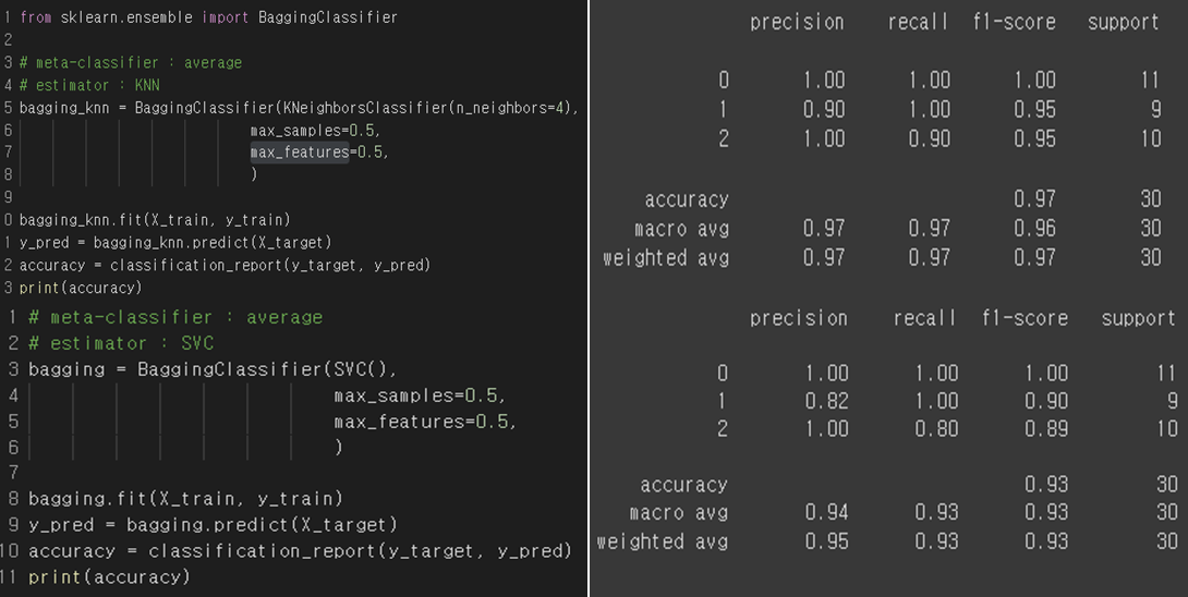
The accuracy of KNN did not change, but the accuracy in SVM is decreased. It can be seen that the model is generalized.
This model shows rather low accuracy on the test set, but when a new data set appears, it will predict much better than the existing single svc model.
Boosting Classifier
Adaboost : Most Famous Boosting algorithm
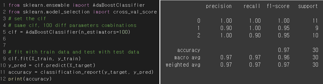
Result Analysis
The boosting method uses a method of increasing the weight of training samples that the previous model underfitted. Therefore, it is useful in solving difficult problems, but has the disadvantage of being sensitive to outliers. We eliminate the outlier when we preprocess the data, the result accuracy is quite high.
Stacking Classifier
Stacked generalization consists in stacking the output of individual estimator and use a classifier to compute the final prediction. Stacking allows to use the strength of each individual estimator by using their output as input of a final estimator.
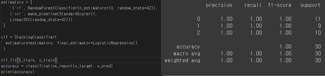
Result Analysis
In this case, I created a stacking classifier by combining Random Forest and Linear Soft Vector Classifier. For final estimator, which is used to combine the estimator and yield the final result, I chose the Logistic Regression model. The result is satisfying, but the stacking methods use huge amount of computing power. So, this method is not exactly appropriate for this simple project.
Voting Classifier
The idea behind the Voting Classifier is to combine conceptually different machine learning classifiers and use a majority vote or the average predicted probabilities (soft vote) to predict the class labels. Such a classifier can be useful for a set of equally well performing models in order to balance out their individual weaknesses.
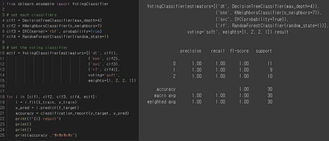
Result Analysis
I combined decision tree, KNN, SVC, and random forest. The result of accuracy is 100% in this case. This is not surprising because each classifier also got almost 100% accuracy score.
5. Conclusion / How to improve
I trained 10 models, such as SVM, KNN, Decision Tree, Random Forest, MLP, CNN, Bagging Classifier, Adaboost, Stacking Classifier, and Voting Classifier. The test data set accuracies of the models are summarized in the table below.
| SVM(rbf) | 0.97 |
| KNN(k = 5) | 0.97 |
| Decision Tree | 1.00 |
| Random Forest | 0.97 |
| MLP | 1.00 |
| CNN | 0.97 |
| Bagging Classifier(SVC) | 0.93 |
| Adaboost | 0.97 |
| Stacking Classifier | 1.00 |
| Voting Classifier | 1.00 |
Reference
https://scikit-learn.org/stable/index.html
https://github.com/rickiepark/handson-ml2/blob/master/10_neural_nets_with_keras.ipynb
'Computer Technology 기록부 > 인공지능 학습 기록부' 카테고리의 다른 글
| ANN Experiment with MNIST Dataset(ENG) (0) | 2023.02.06 |
|---|---|
| Image Data Generation using DCGAN(ENG) (0) | 2023.02.06 |
| Regularization과 Normalization (0) | 2022.02.11 |
| 딥러닝 레이어 이해하기 Embedding Layer, Recurrent layer (0) | 2022.02.09 |
| 딥러닝 레이어 이해하기 linear, Convolution (0) | 2022.02.08 |


댓글